Design concepts
This chapter introduces the reader to a few of the design concepts in MDT.
Protocol
In MDT, the Protocol contains the MRI measurement settings and is, by convention, stored in a protocol file with suffix .prtcl.
In such a protocol file, every row represents an MRI volume, and every column (tab separated) represents a specific protocol setting.
Since every row (within a column) can have a distinct value, this setup automatically enables multi-shell protocol files (just change the b-value per volume/row).
The following is an example of a simple MDT protocol file:
#gx,gy,gz,b
0.000e+00    0.000e+00    0.000e+00    0.000e+00
5.572e-01    6.731e-01    -4.860e-01   1.000e+09
4.110e-01    -5.254e-01   -7.449e-01   1.000e+09
...
And, for a more advanced protocol file:
#gx,gy,gz,Delta,delta,TE,b
-0.00e+0   0.00e+0   0.00e+0  2.18e-2   1.29e-2   5.70e-2   0.00e+0
 2.92e-1   1.71e-1  -9.41e-1  2.18e-2   1.29e-2   5.70e-2   3.00e+9
-9.87e-1  -8.54e-3  -1.60e-1  2.18e-2   1.29e-2   5.70e-2   5.00e+9
...
The header (starting with #) is a single required line with per column the name of that column. The order of the columns does not matter but the order of the header names should match the order of the value columns. MDT automatically links protocol columns to the protocol parameters of a model (see Protocol parameters), so make sure that the columns names are identical to the protocol parameter names in your model.
The pre-provided list of column names is:
- b, the b-values in \(s/m^2\) (\(b = \gamma^2 G^2 \delta^2 (\Delta-\delta/3)\) with \(\gamma = 2.675987E8 \: rads \cdot s^{-1} \cdot T^{-1}\))
- gx, gy, gz, the gradient direction as a unit vector
- Delta, the value for \({\Delta}\) in seconds
- delta, the value for \({\delta}\) in seconds
- G, the gradient amplitude in T/m (Tesla per meter)
- TE, the echo time in seconds
- TR, the repetition time in seconds
Note that MDT expects the columns to be in SI units.
The protocol dependencies change per model and MDT will issue a warning if a required column is missing from the protocol.
A protocol can be created from a bvec/bval pair using the command line, python shell and/or GUI. Please see the relevant sections in Maximum Likelihood Estimation for more details on creating a Protocol file.
Input data
In MDT, all data that is needed to fit a model is stored in a SimpleMRIInputData object.
An instance of this object needs to be created before fitting a model.
Then, during model fitting, the model loads the relevant data for the computations.
The easiest way to instantiate a input data object is by using the function load_input_data().
At a bare minimum, this function requires:
volume_info, a path to the diffusion weighted volumeprotocol, an Protocol instance containing the protocol informationmask, the mask (3d) specifying which voxels to use for the computations
Additionally you can provide noise standard deviation, a gradient deviations file and a dictionary of extra protocol values.
For the noise standard deviation you have the choice to either provide a single value, an ndarray with a value per voxel, or the string ‘auto’.
If ‘auto’ is given, MDT will try to estimate the noise standard deviation from the unweighted volumes.
While this typically works, it is advised to estimate the noise std. manually from air or from noise lines in your k-space.
The gradient deviations is a map specifying how the g vector differs in different areas in the scan.
This can be provided in HCP Wu-Minn format, as a 3x3 matrix per voxel, or as a 3x3 matrix per voxel per volume (i.e. as a (x, y, z, n, 3, 3) matrix for a dataset with n volumes).
With the extra protocol values the user can provide additional protocol values, these can be scalars, vectors, and/or volumes.
If given, these values take precedence over the values in the protocol file.
Dynamic modules
Extending and adapting MDT with new models is made easy using the dynamic library system allowing you to (re)define models anywhere. Users are free to add, remove and modify components and MDT will pickup the changes automatically. See Adding components for more information.
CL code
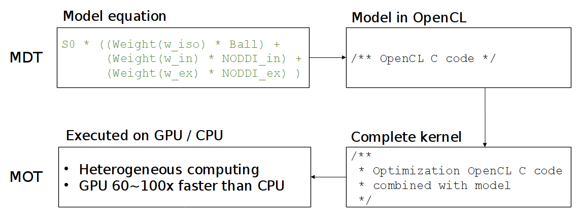
While MDT (and MOT) are programmed in Python, the actual computations are executed using OpenCL. OpenCL is a platform and language specification that allows you to run C-like code on both the processor (CPU) and the graphics cards (GPU). The reason MDT can be fast is since it a) uses a compiled language (OpenCL C) for the computations and b) executes this on the graphics card and/or all CPU cores.
The compartment models in MDT are programmed in the OpenCL C language (CL language from hereon). See (https://www.khronos.org/registry/cl/sdk/1.2/docs/man/xhtml/mathFunctions.html) for a quick reference on the available math functions in OpenCL.
When optimizing a multi-compartment model, MDT combines the CL code of all your compartments into one large function and uses MOT to optimize this function using the OpenCL framework. See this figure for the general compilation flow in MDT:
To support both single and double floating point precision, MDT uses the mot_float_type instead of float and double for most of the variables and function definitions.
During optimization and sampling, mot_float_type is type-defined to be either a float or a double, depending on the desired precision.
Of course this does not limit you to use double and float as well in your code.