Maps visualizer

The MDT maps visualizer is a small convenience utility to visually inspect multiple nifti files simultaneously. In particular, it is useful for quickly visualizing model fitting results.

This viewer is by far not as sophisticated as for example fslview and itksnap, but that is also not its intention. The primary goal of this visualizer is to quickly display model fitting results to evaluate the quality of fit. A side-goal of the viewer is the ability to create reproducible and paper ready figures showing slices of various volumetric maps.

Features include:

• output figures as images (.png and jpg) and as vector files (.svg)
• the ability to store plot configuration files that can later be loaded to reproduce figures
• easily display multiple maps simultaneously

Some usage tip and tricks are:

• Click on a point on a map for an annotation box, click outside a map to disable
• Zoom in by scrolling in a plot
• Move the zoom box by clicking and dragging in a plot
• Add new nifti files by dragging them from a folder into the GUI

The following is a screenshot of the GUI displaying NODDI results of the b1k_b2k MDT example data slices.

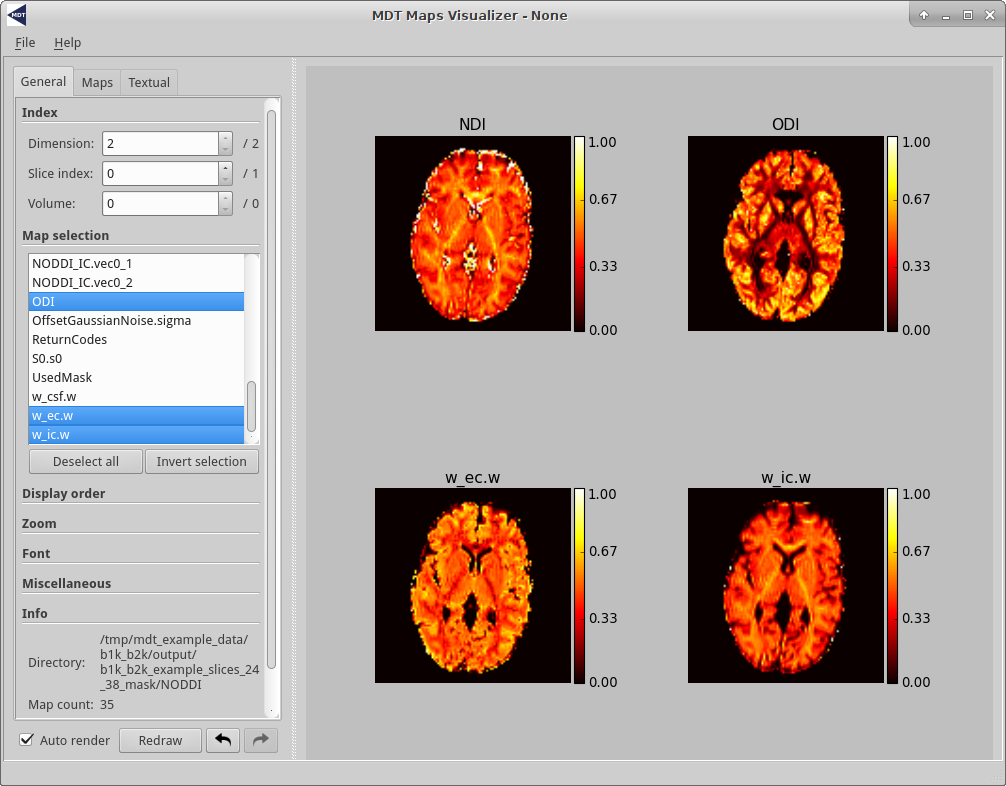
The MDT map visualizer in Linux

The MDT maps visualizer can be started in three ways, from the MDT analysis GUI, from the command line and using the Python API. With the command line, the visualizer can be started using the command mdt-view-maps, for example:

$ mdt-view-maps .

In Windows, one can also type this command in the start menu search bar to load and start the GUI. Using Python, the GUI can be started using the command mdt.view_maps(), for example:

>>> import mdt
>>> mdt.view_maps('output/NODDI')

Finally, using the MDT analyis GUI, the maps visualizer can be started from the menu bar, “File” -> “Maps visualizer”

GUI Layout

The main body of the GUI is split into two parts, the control panel on the left and the display panel on the right. All plot configuration options can be updated using the control panel, which includes things like colormaps, zooming, font sizes, rotations, clipping and more. Changes in the plot settings are automatically reflected in the display panel. This panel shows the current plot using matplotlib as a plotting backend.

On the bottom of the control panel are a few switches to control the rendering of the plots in the display panel. The checkbox “Auto render” disables/enables the automatic rerendering of the plots, allowing you to change multiple settings without rerendering delays. A manual redraw can be forced using the “Redraw” button. The back and forward arrows allow you to undo or redo updates to the plot settings.

When hovering a map, the bottom right of the window shows some basic voxel statistics for the current mouse position. The first tuple ((63, 50) in the example screenshot below), shows the position of the hovered voxel in the current viewport. The second tuple ((63, 50, 0) in the example) shows the absolute position of the hovered voxel inside the nifti file (the two tuples can be different when the map is zoomed in or rotated). Finally, the last item shows the value/intensity of the hovered voxel.

Screenshot of the GUI running in Linux

Control panel

The control panel consists of three tabs, “General”, “Maps” and “Textual”. The first tab contains general options that all apply to the figure in total. For instance, the zoom settings allows you to zoom in on all maps at the same time and the rotate option under miscellaneous rotates all displayed figures.

The second tab is for map specific options, here one can set plot configuration options that apply only to a single map. After having selected the map you wish to change using the drop down box on the top of the panel you can then update all the values in the tab and the changes will be applied to the chosen map. A common thing to change is the “Scale” of the map, which sets the range of the colormap to the defined scale, left empty this will auto-select a good scaling. Another thing that can be set is the “Clipping” which will actively clip the data to be within the defined range.

The last tab of the control panel contains a live text area that allows you to change all plot settings (the general and the map specific) using a text editor. This text box is automatically updated whenever one of the settings on the other tabs changes and vice versa. This text box can be used to, for example, copy paste a configuration from one plot into another to let both reflect the exact same settings. For more information on this feature, please see the next section.

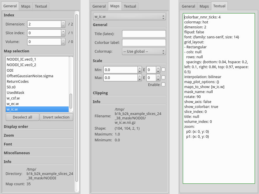
Figure showing the three tabs of the control panel combined into one figure, with the general tab on the left, the map specific options in the center and the textual input tab on the right.

Plot configuration

Any instance of the visualization routine consists of two things, data and a plot configuration. The data is commonly loaded by selecting a directory with maps to load (or, using the Python API, a dictionary with maps). Then, the selected maps or a subset of the maps, are visualized according to the plot configuration. This plot configuration can be configured implicitly by using the “General” and “Maps” tag or explicitly using the “Textual” tab.

The plot configuration is commonly stored as a YAML formatted string that lists the various options as dictionary elements. For example, the following configuration is a configuration for BallStick_r1 model fitting results where we set the zoom and the plot titles using the control panels. As an example, after having followed the analysis getting started guide with the BallStick_r1 model, you could try to copy paste this example configuration in the “Textual” tab in the viewer. It should then update the plot to reflect this configuration.

maps_to_show: [w_ball.w, w_stick.w]
slice_index: 0
zoom:
  p0: {x: 18, y: 4}
  p1: {x: 85, y: 98}
map_plot_options:
  w_ball.w:
    scale: {use_max: true, use_min: true, vmax: 1.0, vmin: 0.0}
    title: Isotropic (w_ball.w)
  w_stick.w:
    scale: {use_max: true, use_min: true, vmax: 1.0, vmin: 0.0}
    title: Anisotropic (w_stick.w)

An alternative way of saving this configuration file is by using the “Export settings” and “Import settings” in the menu. This will provide easy ways of loading and saving the configuration file as a .conf file in YAML format.