Maximum Likelihood Estimation¶

Maximum Likelihood Estimation (MLE), otherwise known as model fitting or model inversion, is one of the core strengths of MDT. Using GPU accelerated fitting routines and a rich library of available models, MDT can fit many types of MRI data within seconds to minutes [Harms2017]. The main workflow is that you load some (pre-processed) MRI data, select a model, and let MDT fit your selected model to the data. The optimized parameter maps are written as nifti files together with variance and covariance estimates and possibly other output maps.

For easy of use with population studies, MDT includes pipelines for the Human Connectome Project (HCP) study, which automatically detects the directory layout of the HCP MGH and HCP WuMinn studies and fit your desired model to (a subset of) the data.

Single dataset fitting is accessible via three interfaces, the Graphical User Interface (GUI), Command Line Interface (CLI) and/or directly using the Python interface.

HCP Pipeline¶

MDT comes pre-installed with Human Connectome Project (HCP) compatible pipelines for the MGH and the WuMinn 3T studies. To run, please change directory to where you downloaded your (pre-processed) HCP data (MGH or WuMinn) and execute:

$ mdt-batch-fit . NODDI

and it will autodetect the study in use and fit your selected model to all the subjects.

For a list of all available models, run the command mdt-list-models.

MDT example data¶

MDT comes pre-loaded with some example data that allows you to quickly get started using the software. This example data can be obtained in the following ways:

GUI: Open the model fitting GUI and find in the menu bar: “Help -> Get example data”.
Command line: Use the command mdt-get-example-data:

$ mdt-get-example-data .

Python API: Use the function mdt.utils.get_example_data():

import mdt
mdt.get_example_data('/tmp')

There are two MDT example datasets, a b1k_b2k dataset and a multishell_b6k_max dataset, both acquired in the same session on a Siemens Prisma system, on the VE11C software line, with the standard product diffusion sequence at 2mm isotropic with GRAPPA in-plane acceleration factor 2 and 6/8 partial fourier (no multiband/simultaneous multi-slice).

The b1k_b2k has a shell of b=1000s/mm^2 and of b=2000s/mm^2 and is very well suited for e.g. Tensor, Ball&Stick and NODDI. In this, the b=1000s/mm^2 shell is the standard Jones 30 direction table, including 6 b0 measurements at the start. The b=2000s/mm^2 shell is a 60 whole-sphere direction set create with an electrostatic repulsion algorithm and has another 7 b0 measurements, 2 at the start of the shell and then one every 12 directions.

The multishell_b6k_max dataset has 6 b0’s at the start and a range of 8 shells between b=750s/mm^2 and b=6000s/mm^2 (in steps of 750s/mm^2) with an increasing number of directions per shell (see De Santis et al., MRM, 2013) and is well suited for CHARMED analysis and other models that require high b-values (but no diffusion time variations).

Graphical interface¶

One of the ways to use MDT for model analysis is by using the Graphical User Interface (GUI). To launch the GUI in Linux and OSX, please open a console and type mdt-gui or MDT to launch the analysis GUI. In Windows one can either open an Anaconda prompt and type mdt-gui or MDT or, alternatively, one can type mdt-gui or MDT in the search bar under the start button to find and launch the GUI.

The following is an example of the GUI running in Linux:

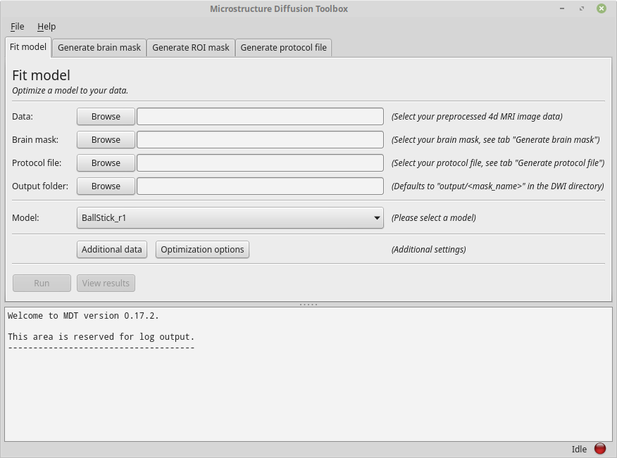
A screenshot of the MDT GUI in Linux.

Using the GUI is a good starting point for model analysis since it guides you through the steps needed for the model analysis. In addition, as a service to the user, the GUI writes Python and Bash script files for most of the actions performed in the GUI. This allows you to use the GUI to generate a coding template that can be used for further processing.

Creating a protocol file¶

As explained in Protocol, MDT stores all the acquisition settings relevant for the analysis in a Protocol file. To create one using the GUI, please go to the tab “Generate protocol file”. On the bottom of the tab you can find the button “Load g & b” which is meant to load a b-vec and b-val file into the GUI. Please click the button and, for the sake of this example, load from the MDT example data folder the b-vec and b-val file of the b1k_b2k dataset. This tab should now look similar to this example:

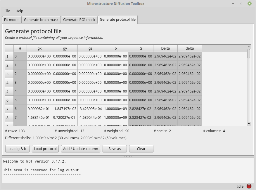
The Protocol tab after loading a bvec and bval file.

Having loaded a b-vec/b-val pair (or a Protocol file), you are presented with a tabular overview of your protocol, with some basic statistics below the table. The table shows you per volume (rows) the values for each of the columns. Columns in gray are automatically calculated or estimated from the other columns. Note that these derived values are there for your convenience and as a check on protocol validity, but cannot be assumed to be strictly correct. For example, in the screenshot above, G, Delta and delta are estimated from the b-values by assuming Delta == delta (this approximation is taken from the NODDI matlab toolbox to be consistent with previous work). Since in reality Delta ~= delta + refocussing RF-pulse length in PGSE, this will underestimate both delta and G. The gray columns are not part of the protocol file and will not be saved.

To add or update a column you can use the dialog under the button “Add / update column”. To remove a column, right click the column header and select the “Remove column” option.

For the sake of this example, please add to the loaded b-vec and b-val files the “Single value” columns “Delta”, “delta”, “TE” and “TR” with values 26.5e-3 seconds, 16.2e-3 seconds, 60e-3 and 7.1 seconds respectively. Having done so, the gray columns for delta and Delta should now turn white (as they no longer are estimated but are actually provided). Your screen should now resemble the following example:

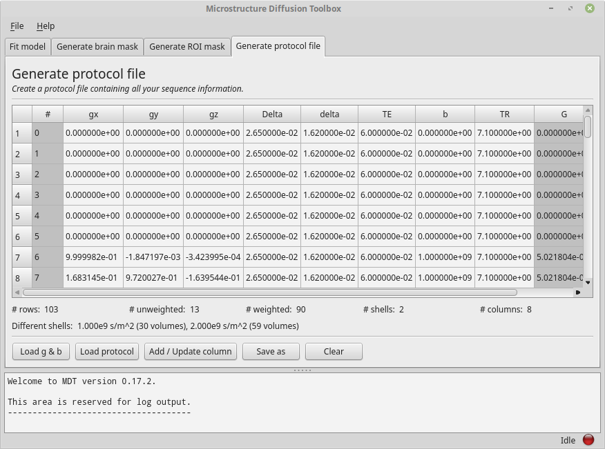
_images/mdt_gui_generate_protocol_filled.png

The Protocol tab after adding various columns.

As an additional check, you could save the protocol as “b1k_b2k_test.prtcl” and compare it to the pre-supplied protocol for comparison (open both in a separate GUI). Alternatively, you could save the file and open with a text editor to study the layout of the protocol file.

Generating a brain mask¶

MDT has some rough functionality for creating a brain mask, similar to the median_otsu algorithm in Dipy. This algorithm is not as sophisticated as for example BET in FSL, therefore we will not go in to much detail here. The mask generating functionality in MDT is merely meant for quickly creating a mask within MDT.

Since the MDT example data comes pre-supplied with a mask (generated by BET), we won’t cover mask generation here. Also, the process is fairly straightforward by just supplying a DWI volume and a protocol.

Generating a ROI mask¶

It is sometimes convenient to run analysis on a single slice (Region Of Interest) before running it whole brain. Using the tab “Generate ROI mask” it is possible to load a whole brain mask and create a new mask where only one slice is used. This ROI mask is just another mask with even more voxels masked.

We do not need this step for the MDT example slices since that dataset is already compressed to two slices.

NODDI estimation example¶

With a protocol and mask ready we can now proceed with model analysis. The first step is to check which devices we are currently using. Please open the runtime settings dialog using the menu bar (typically on the top of the GUI, File -> Runtime settings). This dialog will resemble the following example except that the devices listed will match your system configuration:

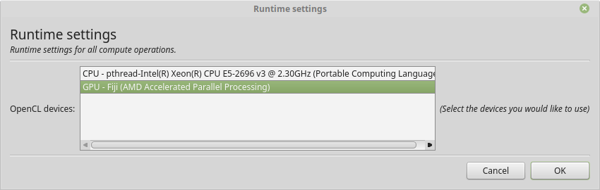
The runtime settings showing the devices MDT can use for the computations.

Typically you only want to select one or all of the available GPU’s (Graphical Processing Units) since they are faster. In contrast, on Apple / OSX the recommendation is to use the CPU since the OpenCL drivers by Apple crash frequently.

Having chosen the device(s) to run on, please open the tab “Fit model” and fill in the fields using the “b1k_b2k” dataset as an example. The drop down menu shows the models MDT can use.

Having filled in all the required fields, select the “NODDI” model, and press “Run”. MDT will now compute your selected model on the data. Please note that for some models, MDT will first compute another model to serve as initialization for your selected model. For instance, when running NODDI, MDT first estimates the BallStick_r1 model to use as initialization for the NODDI model. When the calculations are finished you can click the “View results” button to launch the MDT map viewer GUI for visually inspecting the results. See Maps visualizer for more details on this visualizer.

By default MDT returns a lot of result maps, like various error maps and additional maps like FSL like vector component maps. All these maps are in nifti format (.nii) and can be viewed and opened in any compatible viewer like for example fslview or the Maps visualizer.

In addition to the results, MDT also writes a Python and a Bash script file to a “script” directory next to your DWI file. These script files allow you to reproduce the model fitting using a Python script file or command line.

Estimating any model¶

In general, using the GUI, estimating any model is just a matter of selecting the right model and clicking the run button. Please be advised though that some models require specific protocol values to be present. For example, the CHARMED models requires that the “TE” is specified in the protocol or as a protocol map. MDT will help you by warning you if the available data is not suited for the selected model.

For adding additional data, like protocol maps, a noise standard deviation or a gradient deviations map you can use the button “Additional data”.

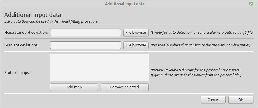
The dialog for adding additional input data.

If you are providing the gradient deviations map, please be advised that this uses the standard set by the HCP Wuminn consortium.

The button “Optimization options” allows you to set some of the Available optimization routines.

Command Line interface¶

After installation a few command line functions are installed to your system. These commands, prefixed with mdt-, allow you to use various functionality of MDT using the command line. For an overview of the available commands, please see: CLI index.

Creating a protocol file¶

As explained in Protocol, MDT stores all the acquisition settings relevant for the analysis in a Protocol file. To create one using the command line, you can use the command mdt-create-protocol. The most basic usage is to create a protocol file from a b-vec and b-val file:

$ mdt-create-protocol data.bvec data.bval

which will generate a protocol file named “data.prtcl”. For a more sophisticated protocol, one can add additional columns using the --<column_name> <value> syntax. For example:

$ mdt-create-protocol d.bvec d.bval --Delta 26.5 --delta delta.txt

which will add both the column Delta to your protocol file (with a static value of 26.5 ms) and the column delta which is read from a file. If a file is given it can either contain a column, row or scalar.

If you have already generated a protocol file and wish to change it you can use the mdt-math-protocol command. This command allows you to change a protocol file using an expression. For example:

$ mdt-math-protocol p.prtcl 'G *= 1e-3; TE = 60e-3; del(TR)' -o new.prtcl

this example command scales G, adds (or replaces) TE and deletes the column TR from the input protocol file and writes the results to a new protocol file.

An example usage in the case of the MDT example data would be the command:

$ cd b1k_b2k
$ mdt-create-protocol b1k_b2k.bvec b1k_b2k.bval \
    --Delta 26.5 \
    --delta 16.2 \
    --TE 60 \
    --TR 7100 \

note that by default the sequence timings are in ms for this function and the elements Delta, delta, TE and TR will automatically be scaled and stored as seconds.

Creating a brain mask¶

MDT has some rough functionality for creating a brain mask, similar to the median_otsu algorithm in Dipy. This algorithm is only meant for generating a rough brain mask and is not as sophisticated as for example BET from FSL.

Creating a mask is possible with the command mdt-create-mask:

$ mdt-create-mask data.nii.gz data.prtcl

which generates a mask named data_mask.nii.gz.

Generating a ROI mask¶

It is sometimes convenient to run analysis on a single slice (Region Of Interest) before running it whole brain. For the example data we do not need this step since that dataset is already compressed to two slices.

To create a ROI mask for your own data you can either use the mdt-create-roi-slice command or the mdt-math-img command. An example with the mdt-create-roi-slice would be:

$ mdt-create-roi-slice mask.nii.gz -d 2 -s 30

here we generate a mask in dimension 2 on index 30 (0-based).

The other way of generating a mask is by using the mdt-math-img command, as a similar example to the previous one:

$ mdt-math-img mask.nii.gz 'a[..., 30]' -o mask_2_30.nii.gz

Also note that since mdt-math-img allows general expressions on nifti files, it can also generate more complex ROI masks.

NODDI estimation example¶

Model fitting using the command line is made easy using the mdt-model-fit command. Please see the reference manual for all switches and options for the model fit command.

The basic usage is to fit for example NODDI on a dataset:

$ cd b1k_b2k
$ mdt-model-fit NODDI \
    b1k_b2k_example_slices_24_38.nii.gz \
    b1k_b2k.prtcl \
    *mask.nii.gz

This command needs at least a model name, a dataset, a protocol and a mask to function. Please note that for some models, MDT will first compute another model to serve as initialization for your selected model. For instance, when running NODDI, MDT first estimates the BallStick_r1 model to use as initialization for the NODDI model. For a list of supported models, please run the command mdt-list-models.

When the calculations are done you can use the MDT maps visualizer (mdt-view-maps) for viewing the results:

$ mdt-view-maps output/BallStick_r1

For more details on the MDT maps visualizer, please see the chapter Maps visualizer.

Estimating any model¶

In principle every model in MDT can be fitted using the mdt-model-fit. Please be advised though that some models require specific protocol values to be present. For example, the CHARMED models requires that the “TE” is specified in your protocol. MDT will warn you if the available data is not suited for the selected model.

Just as in the GUI, it is possible to add additional data like protocol maps, a noise standard deviation or a gradient deviations map to the model fit command. Please see the available switches of the mdt-model-fit command.

Python interface¶

The most direct method to interface with MDT is by using the Python interface. Most actions in MDT are accessible using the mdt namespace, obtainable using:

import mdt

When using MDT in an interactive shell you can use the default dir and help commands to get more information about the MDT functions. For example:

>>> import mdt
>>> dir(mdt) # shows the functions in the MDT namespace
...
>>> help(mdt.fit_model) # shows the documentation a function
...

Creating a protocol file¶

As explained in Protocol, MDT stores all the acquisition settings relevant for the analysis in a Protocol file. The simplest way of creating a Protocol is by using the function create_protocol() to create a Protocol file and object.

To (re-)create the protocol file for the b1k_b2k dataset you can use the following command:

protocol = mdt.create_protocol(
    bvecs='b1k_b2k.bvec', bvals='b1k_b2k.bval',
    out_file='b1k_b2k.prtcl',
    Delta=26.5e-3, delta=16.2-3, TE=60e-3, TR=7.1)

Please note that the Protocol class is a singleton and adding or removing columns involves a copy operation. Also note that we require the columns to be in SI units.

Generating a brain mask¶

MDT has some rough functionality for creating a brain mask, similar to the median_otsu algorithm in Dipy. This algorithm is not as sophisticated as for example BET in FSL, therefore we will not go in to much detail here. The mask generating functionality in MDT is merely meant for quickly creating a mask within MDT.

Creating a mask with the MDT Python interface can be done using the function create_median_otsu_brain_mask(). For example:

mdt.create_median_otsu_brain_mask(
    'b1k_b2k_example_slices_24_38.nii.gz',
    'b1k_b2k.prtcl',
    'data_mask.nii.gz')

which generates a mask named data_mask.nii.gz.

Generating a ROI mask¶

It is sometimes convenient to run analysis on a single slice (Region Of Interest) before running it whole brain. For the example data we do not need this step since that dataset is already compressed to two slices.

Since we are using the Python interface we can use any Numpy slice operation to cut the data as we please. An example of operating on a nifti file is given by:

nifti = mdt.load_nifti('mask.nii.gz')
data = nifti.get_data()
header = nifti.header

roi_slice = data[..., 30]

mdt.write_nifti(roi_slice, header, 'roi_mask.nii.gz')

this generates a mask in dimension 2 on index 30 (be wary, Numpy and hence MDT use 0-based indicing).

NODDI estimation example¶

For model fitting you can use the fit_model() command. This command allows you to optimize any of the models in MDT given only a model, input data and output folder.

The basic usage is to fit for example NODDI on a dataset:

input_data = mdt.load_input_data(
    '../b1k_b2k/b1k_b2k_example_slices_24_38',
    '../b1k_b2k/b1k_b2k.prtcl',
    '../b1k_b2k/b1k_b2k_example_slices_24_38_mask')

inits = mdt.get_optimization_inits('NODDI', input_data, 'output')

mdt.fit_model('NODDI', input_data, 'output',
              initialization_data={'inits': inits})

First, we load the input data (see load_input_data()) with all the relevant modeling information. Second, we try to find a good starting position for our model using the mdt.get_optimization_inits() command. This function returns a dictionary with initialization, fixation and boundary condition information which is suitable for your model and data. Please note that this function only works for models that ship by default with MDT, but due to the general nature of the initialization_data attribute of the fit_model() function you can easily generate your own initialization values.

By default, this model fit function tries to initialize the model with a good starting point using the function mdt.get_optimization_inits(). You can also disable this feature by setting use_cascaded_inits to False, i.e.:

mdt.fit_model('NODDI', input_data, 'output',
              use_cascaded_inits=False)

For precise control of the initialization, you can also find the starting point yourself and initialize the model manually using:

input_data = ...

inits = mdt.get_optimization_inits('NODDI', input_data, 'output')

mdt.fit_model('NODDI', input_data, 'output',
              use_cascaded_inits=False,
              initialization_data={'inits': inits})

When the calculations are done you can use the MDT maps visualizer for viewing the results:

mdt.view_maps('../b1k_b2k/output/BallStick_r1')

Full example¶

To summarize the code written above, here is a complete and ease of use MDT model fitting example:

import mdt

protocol = mdt.create_protocol(
    bvecs='b1k_b2k.bvec', bvals='b1k_b2k.bval',
    out_file='b1k_b2k.prtcl',
    Delta=26.5e-3, delta=16.2-3, TE=60e-3, TR=7.1)

input_data = mdt.load_input_data(
    'b1k_b2k_example_slices_24_38',
    'b1k_b2k.prtcl',
    'b1k_b2k_example_slices_24_38_mask')

mdt.fit_model('NODDI', input_data, 'output')

Estimating any model¶

In principle every model in MDT can be fitted using the model fitting routines. Please be advised though that some models require specific protocol values to be present. For example, the CHARMED models requires that the “TE” is specified in your protocol. MDT will help you by warning you if the available data is not suited for the selected model.

To add additional data to your model computations, you can use the additional keyword arguments to the load_input_data() command.

Fixing parameters¶

To fix parameters, as for example fibre orientation parameters, one can use the initialization_data keyword of the fit_model() command. This keyword allows fixing and initializing parameters just before model optimization and sampling. The following example shows how to fix the fibre orientation parameters of the NODDI model during optimization:

theta, phi = <some function to generate angles>

mdt.fit_model('NODDI',
    ...
    initialization_data={
        'fixes': {'NODDI_IC.theta': theta,
                  'NODDI_IC.phi': phi}
    })

The syntax of the initialization_data is:

initialization_data = {'fixes': {...}, 'inits': {...}}

where both fixes and inits are dictionaries with model parameter names mapping to either scalars or 3d/4d volumes. The fixes indicates parameters that will be fixed to those values, which will actively exclude those parameters from optimization. The inits indicate initial values (starting position) for the parameters.

Available optimization routines¶

MDT features GPU accelerated optimization routines, carefully selected for their use in microstructure MRI imaging [Harms2017]. For reusability, these optimization routines are available in the Multithreaded Optimization Toolbox (MOT). This optimization toolbox contains various optimization routines programmed in OpenCL for optimal performance on both CPU and GPU. The following optimization routines are available to MDT:

Powell [Powell1964] (wiki)
Levenberg-Marquardt [Levenberg1944], (wiki)
Nelder-Mead simplex [Nelder1965], (wiki)
Subplex [Rowan1990]

the number of iterations of each of these routines can be controlled by a variable named patience which sets the number of iterations to \(p * (n+1)\) where \(p\) is the patience and \(n\) the number of parameters to be fitted. By setting the patience indirectly we can implicitly account for model complexity.

By default, MDT uses the Powell routine for all models, although with some models a different routine might perform better for a specific model. We advice experimenting with the different routines to see which performs best for your model.

Setting the routine¶

From within the graphical interface, the options can be set using the Optimization Options button in the model fit tab. Showing you a frame similar to:

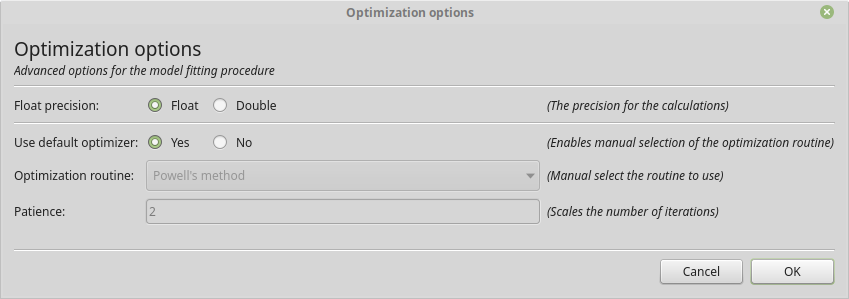
The graphical dialog to setting the optimization options.

Using the command line the same options can be set using --method and --patience, as:

$ cd b1k_b2k
$ mdt-model-fit \
    ... \
    --method Powell
    --patience 2

Using the Python API the options are specified as:

mdt.fit_model(
    ...,
    method='Powell',
    optimizer_options={'patience': 2}
)

References